Understanding One-Way ANOVA in R: A Step-by-Step Tutorial
ANOVA
Post-Hoc Analysis
Tukey test
Density plot
QQ plot
Scatter plot
Author
Farhan Khalid
Published
January 30, 2025
Keywords
One-Way ANOVA, Iris dataset, Hypothesis Testing, Assumption Checking, Normality, Homogeneity of Variance, Independence, Post-Hoc Tests, Tukey’s HSD, Effect Size, Eta-squared, Data Visualization, Density Plots, Q-Q Plots, Scatter Plots, Levene’s Test, Welch’s ANOVA, R Packages, car package, ggplot2, effectsize
One-Way Analysis of Variance (ANOVA)
One-Way ANOVA is a statistical method used to compare means across three or more independent groups. In this tutorial, we’ll use R’s built-in iris dataset to demonstrate the complete workflow.
1. Define the Research Question & Hypotheses
Research Question:
Do different iris flower species have significantly different sepal lengths?
Hypotheses:
- \(H_0\): \(\mu_{setosa} = \mu_{versicolor} = \mu_{virginica}\)
- \(H_1\): At least one species has a different mean sepal length
Independent Variable: Species (3 levels: setosa, versicolor, virginica)
Dependent Variable: Sepal.Length (continuous)
3. Check Assumptions
Independence
While we assume independence in the iris dataset, in practice this is ensured through proper experimental design.
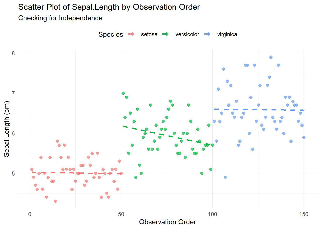
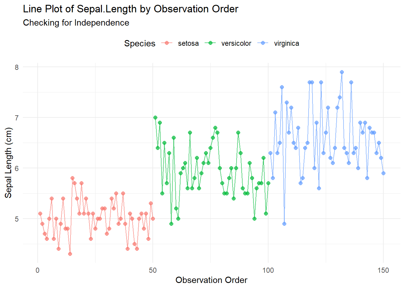
You can visually examine indepedence by creating a scatter plot and line plot.
# Create a scatter plot to visualize independenceggplot(iris, aes(x =seq_along(Sepal.Length), y = Sepal.Length, color = Species)) +geom_point(size =2, alpha =0.7) +# Add pointsgeom_smooth(method ="lm", se =FALSE, linetype ="dashed") +# Add trend lineslabs(title ="Scatter Plot of Sepal.Length by Observation Order",subtitle ="Checking for Independence",x ="Observation Order",y ="Sepal Length (cm)" ) +theme_minimal() +theme(legend.position ="top")
# Create a line plot to visualize independenceggplot(iris, aes(x =seq_along(Sepal.Length), y = Sepal.Length, color = Species)) +geom_line(size =0.5, alpha =0.7) +# Add linesgeom_point(size =2, alpha =0.7) +# Add pointslabs(title ="Line Plot of Sepal.Length by Observation Order",subtitle ="Checking for Independence",x ="Observation Order",y ="Sepal Length (cm)" ) +theme_minimal() +theme(legend.position ="top")
Interpretation:
Clustering by Species: The iris dataset is structured such that observations are grouped by species (e.g., first 50 rows = setosa, next 50 = versicolor, last 50 = virginica). This explains the three distinct horizontal bands in the scatter plot:
Setosa: Lower sepal lengths (~4–6 cm) clustered at observations 1–50.
Versicolor: Medium sepal lengths (~5–7 cm) at observations 51–100.
Virginica: Higher sepal lengths (~6–8 cm) at observations 101–150.
No Trend Within Species: Within each species group (e.g., setosa from 1–50), the points appear randomly scattered vertically (no increasing/decreasing pattern).
Conclusion for Independence:
The clustering is due to the dataset’s inherent structure (sorted by species), not a violation of independence.
Observations within each species group show no systematic trend over the observation order, supporting independence.
$setosa

    Shapiro-Wilk normality test

data:  X[[i]]
W = 0.9777, p-value = 0.4595


$versicolor

    Shapiro-Wilk normality test

data:  X[[i]]
W = 0.97784, p-value = 0.4647


$virginica

    Shapiro-Wilk normality test

data:  X[[i]]
W = 0.97118, p-value = 0.2583
Interpretation: All p-values > 0.05 ⇒ Data appears normally distributed in each group.
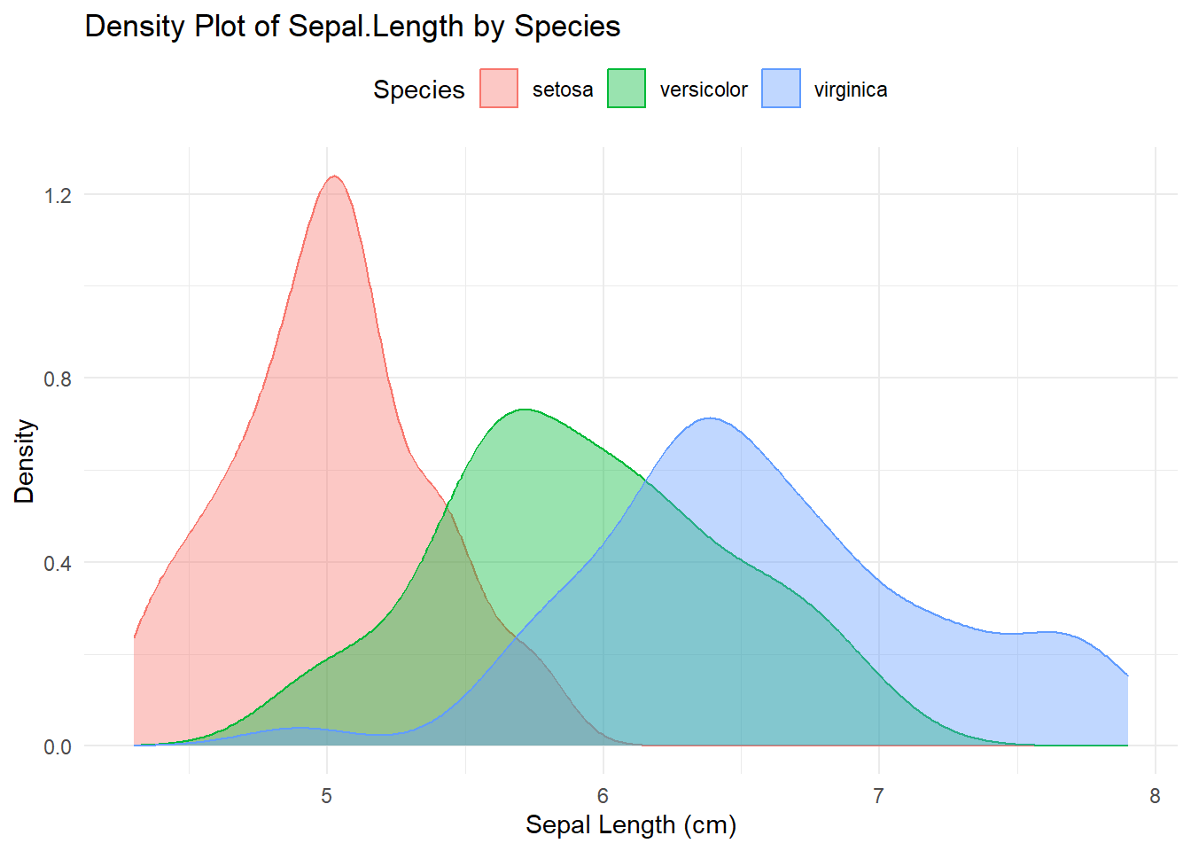
Density Plot for Normality Check
A density plot will help you visualize the distribution of Sepal.Length for each species. If the data is normally distributed, the density curve will resemble a bell-shaped curve.
# Create a density plot for Sepal.Length by Speciesggplot(iris, aes(x = Sepal.Length, color = Species, fill = Species)) +geom_density(alpha =0.4) +# Add density curves with transparencylabs(title ="Density Plot of Sepal.Length by Species",x ="Sepal Length (cm)",y ="Density" ) +theme_minimal() +theme(legend.position ="top")
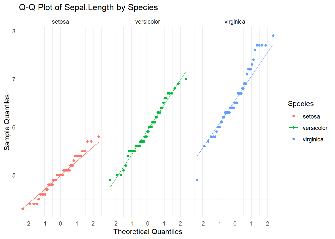
Q-Q Plot for Normality Check
A Q-Q plot is another way to visually check for normality. It compares the quantiles of the data to the quantiles of a theoretical normal distribution. If the points fall approximately along the reference line, the data is normally distributed.
# Create Q-Q plots for Sepal.Length by Speciesggplot(iris, aes(sample = Sepal.Length, color = Species)) +stat_qq() +stat_qq_line() +facet_wrap(~ Species) +# Separate plots for each specieslabs(title ="Q-Q Plot of Sepal.Length by Species",x ="Theoretical Quantiles",y ="Sample Quantiles" ) +theme_minimal()
Homogeneity of Variance
Critical Step
If Levene’s test indicates unequal variances (p < 0.05), use Welch’s ANOVA (oneway.test()) instead of classic ANOVA.
leveneTest(Sepal.Length ~ Species, data = iris)
Levene's Test for Homogeneity of Variance (center = median)
       Df F value   Pr(>F)
group   2  6.3527 0.002259 **
      147
---
Signif. codes:  0 '***' 0.001 '**' 0.01 '*' 0.05 '.' 0.1 ' ' 1
Interpretation:
Null Hypothesis (H₀): The variances across the groups (iris species) are equal.
Alternative Hypothesis (H₁): The variances across the groups are not equal.
The p-value (0.002259) is less than the common significance level of α = 0.05. This means we reject the null hypothesis and conclude that there is significant evidence that the variances of sepal lengths are not equal across the three iris species (setosa, versicolor, and virginica).
Implications for ANOVA:
The assumption of homogeneity of variance is violated. While ANOVA is somewhat robust to this violation, especially with balanced sample sizes, it is important to consider this result when interpreting the ANOVA findings.
If the violation is severe, you might consider using a Welch’s ANOVA (which does not assume equal variances) or transforming the data to stabilize variances.
Caution
Violations of ANOVA assumptions (e.g., non-normality) may require non-parametric alternatives like the Kruskal-Wallis test.
4. Compute ANOVA
anova_model <-aov(Sepal.Length ~ Species, data = iris)anova(anova_model)
Analysis of Variance Table

Response: Sepal.Length
           Df Sum Sq Mean Sq F value    Pr(>F)
Species     2 63.212  31.606  119.26 < 2.2e-16 ***
Residuals 147 38.956   0.265
---
Signif. codes:  0 '***' 0.001 '**' 0.01 '*' 0.05 '.' 0.1 ' ' 1
Output Interpretation:
- F(2, 147) = 119.26
- p < 2.2e-16 ⇒ Significant difference exists between species
Did You Know?
The F-statistic in ANOVA compares between-group variance to within-group variance.
5. Interpret Results
The significant p-value (p < 0.001) indicates we reject \(H_0\) - at least two species have different mean sepal lengths.
6. Post-Hoc Analysis (Tukey’s HSD)
TukeyHSD(anova_model)
  Tukey multiple comparisons of means
    95% family-wise confidence level

Fit: aov(formula = Sepal.Length ~ Species, data = iris)

$Species
                      diff       lwr       upr p adj
versicolor-setosa    0.930 0.6862273 1.1737727     0
virginica-setosa     1.582 1.3382273 1.8257727     0
virginica-versicolor 0.652 0.4082273 0.8957727     0
Key Findings:
- All pairwise comparisons show significant differences (p < 0.001)
- Largest difference: virginica vs setosa (mean difference = 1.582)
Why Use Tukey’s HSD?
Tukey’s Honest Significant Difference test controls the family-wise error rate, reducing false positives in multiple comparisons.
7. Effect Size Calculation
eta_squared(anova_model)
For one-way between subjects designs, partial eta squared is equivalent
  to eta squared. Returning eta squared.
# Effect Size for ANOVA

Parameter | Eta2 |       95% CI
-------------------------------
Species   | 0.62 | [0.54, 1.00]

- One-sided CIs: upper bound fixed at [1.00].
Interpretation:
η² = 0.62 ⇒ 62% of variance in sepal length is explained by species (large effect).