In this document, we demonstrate how to perform a one-sample t-test in R to determine whether the mean of a single sample significantly differs from a hypothesized value. Specifically, we investigate whether the average miles per gallon (mpg) in the mtcars dataset is statistically different from 20. The one-sample t-test is a parametric test that is used when the data are assumed to be normally distributed and the observations are independent.
Hypotheses
For the one-sample t-test, the hypotheses are defined as follows:
Null Hypothesis (H₀): The population mean is equal to the hypothesized value, i.e., μ = μ₀ (in this case, μ₀ = 20).
Alternative Hypothesis (H₁): The population mean is not equal to the hypothesized value, i.e., μ ≠ μ₀.
Performing the One-Sample t-Test
We use the built-in t.test function in R to perform the one-sample t-test on the mpg variable of the mtcars dataset.
# Perform one-sample t-test on 'mpg' with the hypothesized mean of 20 t_test_result <-t.test(mtcars$mpg, mu =20) t_test_result
    One Sample t-test

data:  mtcars$mpg
t = 0.08506, df = 31, p-value = 0.9328
alternative hypothesis: true mean is not equal to 20
95 percent confidence interval:
 17.91768 22.26357
sample estimates:
mean of x
 20.09062
Sample Size Considerations
While the t-test is robust to moderate deviations from normality, very small sample sizes can lead to misleading conclusions. Consider using non-parametric alternatives (e.g., the Wilcoxon signed-rank test) when in doubt.
Assumption of Normality
Ensure that the data are approximately normally distributed. This assumption is particularly important when the sample size is small (n < 30). If the normality assumption is violated, the test results may not be reliable.
Outliers
Outliers can greatly influence the mean and variance. Before running the test, inspect the data for outliers and consider whether they should be addressed or removed.
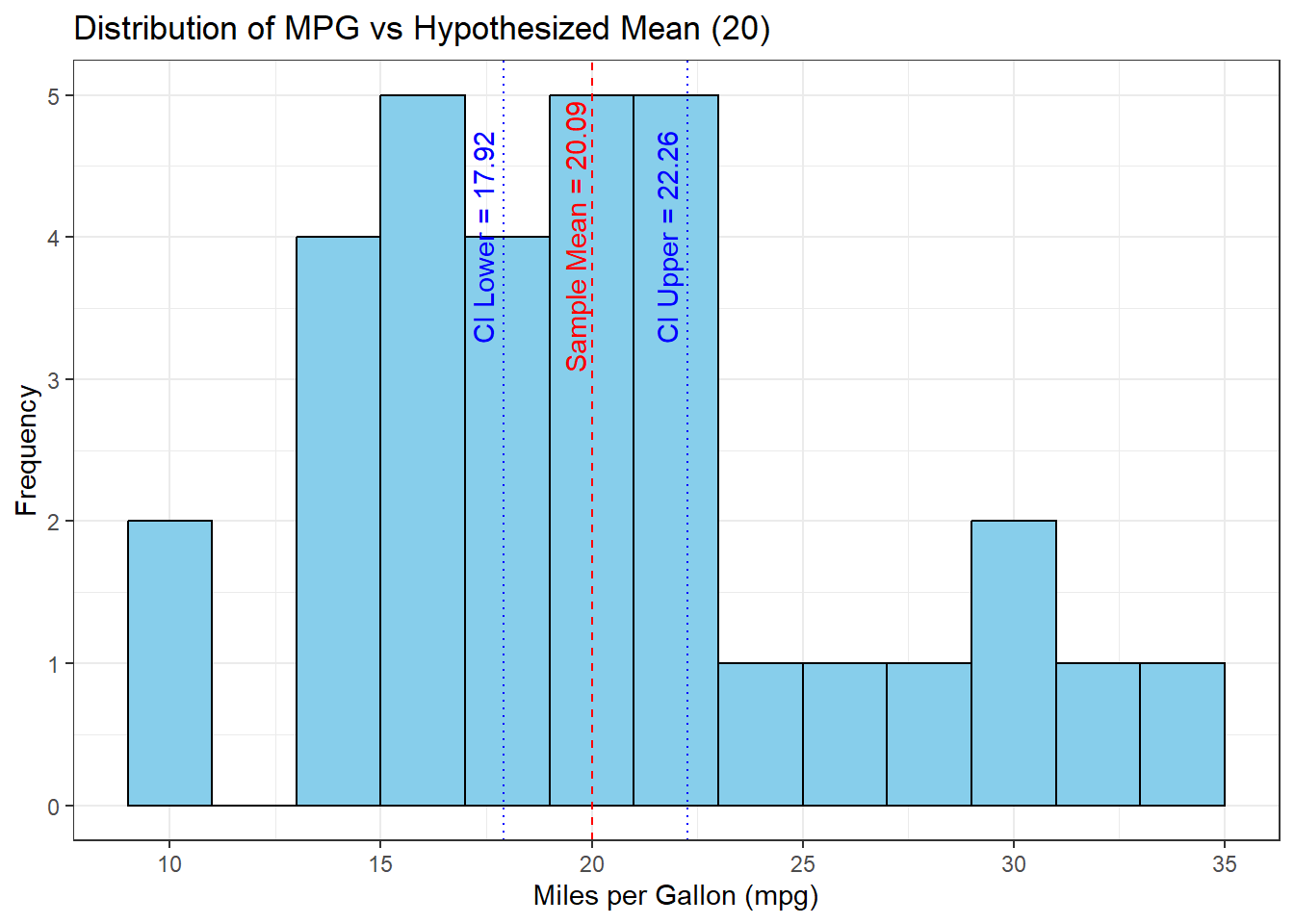
Visualization of the Data Distribution
To better understand the distribution of mpg values relative to the hypothesized mean, we can visualize the data using a histogram. A vertical dashed red line indicates the hypothesized mean of 20.
# Plot histogram of mpg with a vertical line at the hypothesized mean (20)ggplot(mtcars, aes(x = mpg)) +geom_histogram(binwidth =2, fill ="skyblue", color ="black") +geom_vline(xintercept =20, color ="red", linetype ="dashed") +geom_vline(xintercept = t_test_result$conf.int[1], color ="blue", linetype ="dotted") +geom_vline(xintercept = t_test_result$conf.int[2],color ="blue",linetype ="dotted") +labs(title ="Distribution of MPG vs Hypothesized Mean (20)",x ="Miles per Gallon (mpg)",y ="Frequency") +annotate("text", x = t_test_result$estimate, y =4, label =paste("Sample Mean =", round(t_test_result$estimate, 2)),color ="red", angle =90, vjust =-0.5) +annotate("text", x = t_test_result$conf.int[1], y =4,label =paste("CI Lower =", round(t_test_result$conf.int[1], 2)),color ="blue",angle =90, vjust =-0.5) +annotate("text", x = t_test_result$conf.int[2], y =4, label =paste("CI Upper =", round(t_test_result$conf.int[2], 2)), color ="blue", angle =90, vjust =-0.5) +theme_bw()
Interpretation of Results
The results of the one-sample t-test are interpreted as follows:
t-Statistic and Degrees of Freedom:
The computed t-statistic is 0.08506 with 31 degrees of freedom. This near-zero t-value suggests that the difference between the sample mean (20.09) and the hypothesized mean (20) is negligible when compared to the variability in the data.
p-Value:
The p-value associated with the test is 0.9328, which is substantially higher than the conventional alpha level of 0.05. A high p-value indicates that there is insufficient evidence to reject the null hypothesis. Thus, we conclude that there is no statistically significant difference between the sample mean and the hypothesized value.
Confidence Interval:
The 95% confidence interval for the population mean is given as (17.92, 22.26). This interval encompasses the hypothesized mean of 20, further supporting the conclusion that the true mean is not significantly different from 20.
Confidence Interval Interpretation
The 95% confidence interval provides a range of plausible values for the population mean. If the hypothesized mean falls within this interval, it suggests that there is no significant difference between the observed mean and the hypothesized value.
In summary, the statistical analysis indicates that the observed average mpg of approximately 20.09 is not significantly different from the hypothesized value of 20.
Conclusion
The one-sample t-test conducted on the mtcars dataset, with a hypothesized mean of 20 for the miles per gallon (mpg) variable, yielded a t-statistic of 0.08506 with 31 degrees of freedom and a p-value of 0.9328. These results indicate that there is no statistically significant difference between the sample mean (approximately 20.09) and the hypothesized value. Moreover, the 95% confidence interval for the true mean, ranging from 17.92 to 22.26, includes the hypothesized value of 20. Consequently, we do not have sufficient evidence to reject the null hypothesis, supporting the conclusion that the true mean mpg is consistent with the hypothesized value of 20.