Learn how to set up an efficient data analysis workflow in RStudio. This tutorial covers creating projects, using RMarkdown for reporting, and organizing scripts effectively.
Author
Farhan Khalid
Published
November 28, 2024
Keywords
RStudio workflow tutorial, Setting up projects in RStudio, Organizing R scripts, RMarkdown reporting guide, Efficient data analysis in R, R programming best practices, Automating data analysis
Efficiency and organization are key to successful data analysis. RStudio, the integrated development environment (IDE) for R, offers tools that streamline the data analysis process. This tutorial will guide you through setting up a structured workflow in RStudio, covering projects, script organization, and report generation with RMarkdown.
Why Build a Workflow?
A good workflow in RStudio ensures: - Organized scripts and files for easy access and collaboration. - Reproducibility of your analysis. - Faster and more efficient work with minimal errors.
Step 1: Setting Up an RStudio Project
What is an RStudio Project?
An RStudio Project is a self-contained workspace. It keeps all your files, scripts, and outputs organized in one folder.
Creating a New Project
Open RStudio.
Navigate to File > New Project.
Choose one of the following options:
New Directory: Create a new folder for your project.
Existing Directory: Use an existing folder.
Name your project and select a location on your computer.
Click Create Project.
Benefits of Using Projects
Automatically sets the working directory.
Keeps files and outputs organized.
Helps maintain reproducibility by isolating environments for different analyses.
Step 2: Organizing Your Workflow
Folder Structure
Organize your project folder for clarity and efficiency. A typical folder structure:
my_project/
|-- data/       # Raw and processed data files
|-- scripts/    # R scripts for analysis
|-- output/     # Results, plots, and reports
|-- README.md   # Project documentation
Script Organization
Divide your scripts based on tasks:
Data Import: Load raw data into R.
Data Cleaning: Process and clean the data.
Analysis: Perform statistical analysis or modeling.
# Save cleaned datawrite.csv(x = data, "cleaned_data.csv")
Step 3: Writing Reports with RMarkdown
What is RMarkdown?
RMarkdown allows you to create dynamic reports that combine code, results, and narrative in a single document.
Creating a New RMarkdown File
Go to File > New File > RMarkdown.
Fill in the title, author, and output format (HTML, PDF, or Word).
Click OK to create the file.
Basic Structure of RMarkdown
Run the document using the Knit button in RStudio. The output will include text, code, and results.
Step 4: Automating Workflow with Scripts
Using source() to Run Scripts
Organize your scripts into separate files and use source() to run them sequentially. For example:
# Master script to execute all stepssource("scripts/01_import_data.R")source("scripts/02_clean_data.R")source("scripts/03_analysis.R")source("scripts/04_visualizations.R")
Step 5: Best Practices for Efficiency
Version Control: Use Git and GitHub to track changes to your code.
Documentation: Add comments and README files to explain your workflow.
Reproducibility: Use R scripts and RMarkdown to ensure analyses can be replicated.
Example: Complete Workflow with mtcars Dataset
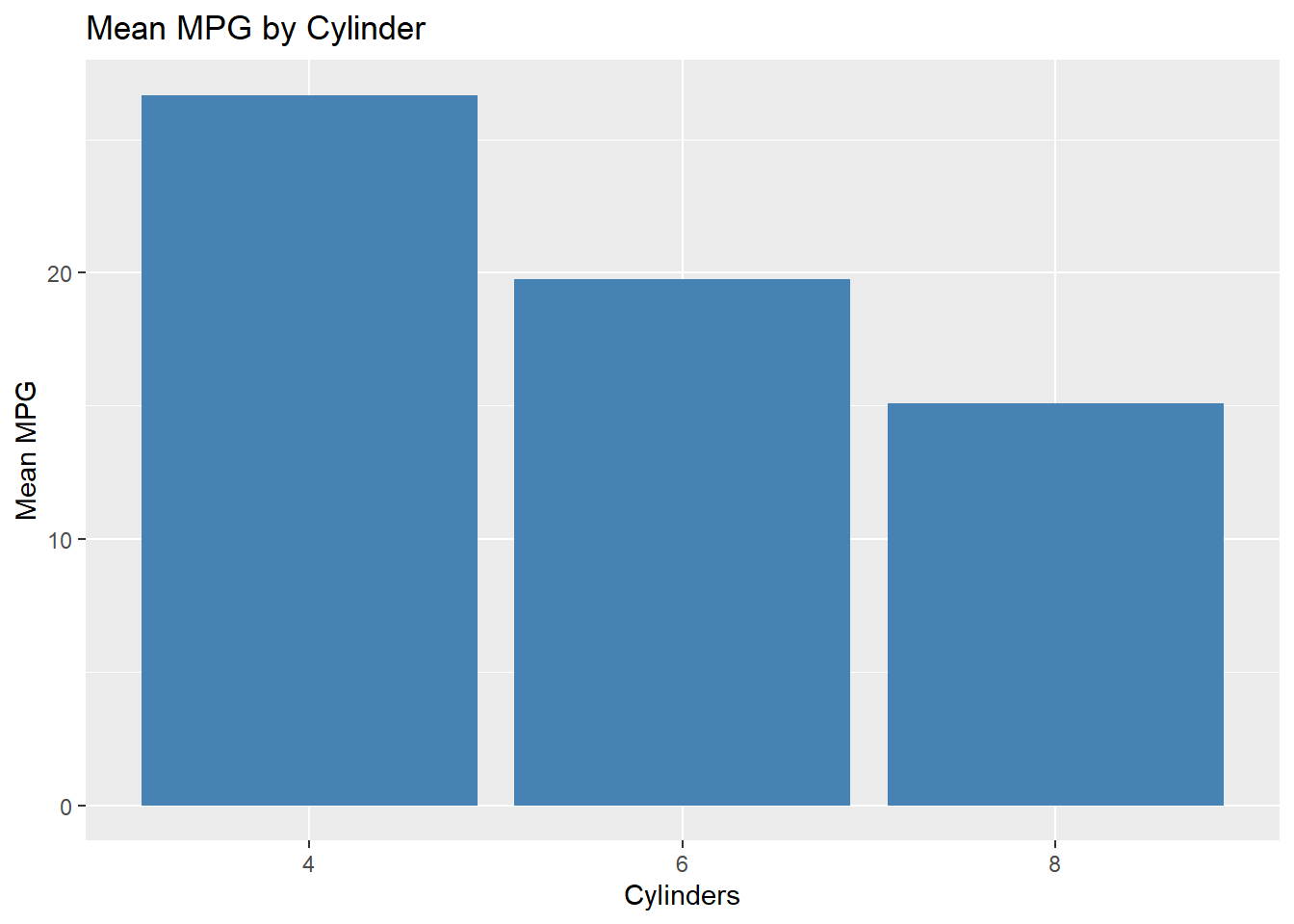
Below is a complete example using the mtcars dataset.
# Bar plot of mean MPG by cylinderggplot(analysis, aes(x = cyl_factor, y = mean_mpg)) +geom_bar(stat ="identity", fill ="steelblue") +labs(title ="Mean MPG by Cylinder", x ="Cylinders", y ="Mean MPG")
Step 5: Reporting
In an RMarkdown document:
Include the code for each step.
Add explanations and results.
Knit the document to HTML for sharing.
Conclusion
By setting up a structured workflow in RStudio, you can make your data analysis process efficient, organized, and reproducible. Start by creating a project, organizing scripts, and using RMarkdown for reporting. Incorporating these best practices into your workflow will save time and improve the quality of your analyses.